論文筆記：A Joint Management Middleware to Improve Training Performance of DLRM with SSDs

ABSTRACT

As the sizes and variety of training data scale over time, data preprocessing is becoming an important performance bottleneck for training deep recommendation systems. This challenge becomes more serious when training data is stored in Solid-State Drives (SSDs). Due to the access behavior gap between recommendation systems and SSDs, unused training data may be read and filtered out during preprocessing. This work advocates a joint management middleware to avoid reading unused data by bridging the access behavior gap. The evaluation results show that our middleware can effectively improve the performance of the data preprocessing phase so as to boost training performance.

INTRODUCTION

Deep recommendation systems are widely adopted to improve user experience across various web services, such as entertainment or e-commerce services. As the sizes and variety of training data grow, the performance bottleneck of recommendation model training gradually shifts from the model training phase to the data preprocessing and ingestion phase.

For example, during model training, more than 56% of GPU cycles were idle and waiting for CPUs to handle training data preprocessing .

We show that, due to the access behavior gap between recommendation model training and SSDs, a significant amount of the data preprocessing phase is spent on reading and filtering unused training data. To improve training performance by minimizing the needs of reading and preprocessing unused data, this work aims to bridge the access behavior gap by advocating a joint management middleware between a GPU-based recommendation training systems and SSDs.

The industry, such as Facebook, Baidu and Google, have adopted deep recommendation models to recommend e-commerce products to each users. Recommendation models comprise:

• Fully-Connected (FC) Layers: Handle dense features
• Embedding-table Layers: Look up the categorical features (usually represented by sparse vectors)

To improve the inference performance, several previous works focus on co-designing recommendation models with various accelerators (e.g., GPUs, TPU-like devices, or in-storage processors).

In addition to inference, improving the performance of model training on large-scale datasets is crucial to the success of products supported by deep recommendation models. Generally, there are two key phases for training:

1. data preprocessing phase: transforms raw data from storage devices to materialized tensor data
2. feature training phase: trains tensor data.

To support massive scale feature training, Baidu proposes a distributed GPU hierarchical parameter server. Aiming at improving the performance of feature training, cDLRM prefetches embedding tables from the host memory to GPU memory at runtime. In addition to feature training, as the sizes and variety of training data scale all the time, Facebook performs an end-to-end analysis in 2021 and shows that the data preprocessing phase gradually becomes the performance bottleneck of recommendation model training.

Industrial recommendation models require tens of petabytes of training data, and are constantly growing all the time. An ever-increasing memory capacity is required to hold all training data in memory. However, Dynamic Random Access Memory (DRAM) faces the scaling challenge and also the average DRAM price has increased several times in recent years.

A practical and cost-effective system configuration for a recommendation system is to cache the most recently used training data in DRAM to enjoy its fast response time, and store all training data in the flash-based SSDs to save the deploy cost.

Due to the design of flash cells, SSDs mainly suffer from limited lifetime and the lifetime becomes shorter when storing more data bits in a cell. Besides, SSDs can only update data out-of-place because data in the flash page shall be erased before written new data in it, but the erase granularity is around dozens times larger than a flash page (please find more details in Section 2.1.2). The out-of-place update means the data shall be read out from the flash page, updated and written to a new flash page. To make SSDs easily compatible with any systems, SSDs adopt the Flash Translation Layer (FTL) to hide these constrains from host systems. FTL comprises a wear leveler to level write accesses on all cells to avoid wearing out some cells earlier, and an address mapper to keep track of the address of the updated data without the intervention from host systems. FTL is a double-edged sword, managing SSDs without host intervention but suffering from weak integration between applications.

Based on our investigation, the access behavior gap between recommendation model training and SSDs may increase the time of reading training data from SSDs during data preprocessing phases. The access behavior gap is that recommendation systems read out whole features during the data preprocessing phase, but the data arrangement of SSDs is not aware of this access behavior and mixes key-value items belonging to different features in the same flash page. Under this access behavior gap, unused key-value items will be read from SSDs, increasing the overall read time while incurring wasted SSD bandwidth. To mitigate the data movement overhead, this paper proposes a middleware, namely rec-aware SSD data arranger, to manage SSDs by taking into account the behavior of recommendation model training. In particular, the proposed middleware comprises (1) a rec-aware data merger to pro-actively merge data belonging to the same feature without seriously hurting SSD’s lifetime, and (2) a rec-aware data pinner to smartly pin data in the write buffer to enhance SSD’s bandwidth utilization. The evaluation results show that our rec-aware SSD data arranger reduces the overall read time by 20%~38% over that of the Log-Structured Merge-Tree (LSM) based strategy adopted in Baidu’s recommendation systems. Our read throughput results are within 12% of the optimal case.

BACKGROUND AND MOTIVATION

2.1 Background

2.1.1 Data Preprocessing of Recommendation Training Systems

Recommendation systems suggest relevant contents to users by leveraging a large-scale training data corpus, such as the online shopping history or the rating of movies. Recommendation models are trained with relevant data stored in storage devices. However, training data read from storage devices cannot be naively fed into trainers (e.g. GPUs or TPUs). One of the reason is that training data will usually be compressed or serialized before storing on storage devices. The data preprocessing design is widely adopted (e.g., Facebook and Google) to extract and transform training data to tensor data that is subsequently ingested into trainers.

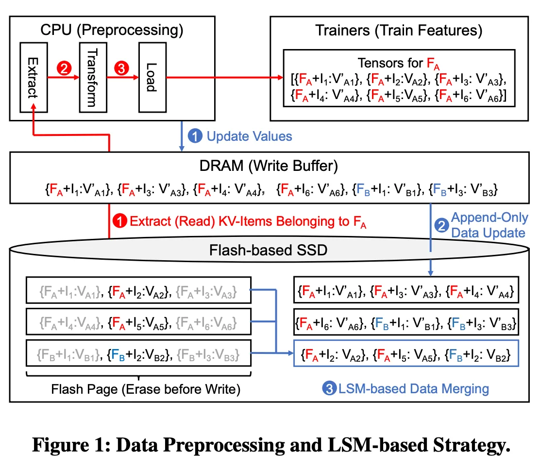
A conceptual data flow of data preprocessing is shown in Figure 1. A recommendation model is trained using multiple features. Each feature is associated with multiple key-value items (or KV-items for short), where each key represents an item and its value indicates the correlation between the item and the feature.

For example, the average book ratings of users can be one of the feature, and each book item with its average ratings is stored as a KV-item. Assuming feature A ($F_A$) is selected for feature training in Figure 1. CPU reads out raw data (including all items and values) belonging to $F_A$ from storage devices (❶). However, due to mismatching formats, extra data including invalid or unused data will also be read out from storage devices (Details of extra data are introduced in Section 2.1.2). During the extraction stage (❷), CPU filters out the data belonging to unused features, and group KV-items for each feature. In the transformation stage (❸), each value will be transformed to the suitable format based on trainers’ requirements (e.g., sorting or normalizing floating numbers). Finally, features will be batched as tensors and loaded to trainers.

2.1.2 Solid-State Drives (SSDs)

With the advancement of manufacturing technology, die costs and the performance of flash-based SSDs have been improved year-by-year.

In the rest of this paper, SSDs represent flash-based SSDs. SSDs are widely deployed in recommendation systems as the storage backend. In contrast to Hard Disk Drives (HDDs) which can update data in-place, SSDs shall update data out-of-place. Generally, the in-place update operation is realized by executing an erase operation to remove the old data and then running a write operation to write new data at the same place. However, due to the characteristic of flash cells, an erase operation cannot erase only one flash page, a minimum read/write granularity for SSDs, because the minimum erase granularity is a flash block, dozens times larger than a flash page.

Without executing erase operations, a common way to update data in SSDs is to do the Read-Modify-Write (RMW) operation, that is to read out flash pages containing the old data, modify all old data to new data, and write all modified flash pages to other free space. With using RMW operations to update data, the minimum update granularity shall align with the flash page size (e.g., 16KB), even when an SSD controller intends to update only few bytes (e.g., 4 Bytes for each value) of data in a flash page. This exaggerated update amplification seriously hurts the lifetime of SSDs. Although systems configure a portion of the DRAM as a write buffer to collect updates, the update amplification can not be effectively alleviated, especially when the capacity of training data scales up.

To alleviate the lifetime issues caused by updating training data, systems usually employ the append-only Log-Structured Merge-Tree (LSM) based strategy. The bottom part of Figure 1 provides the conceptual procedures of the append-only LSM-based strategy. All updated training data will be buffered in the write buffer before being updated to SSDs (❶).

For example, $\{F_A + I_1 : V'_{A1}\}$ in the write buffer denotes that the value of item 1 ($I_1$) belonging to feature A ($F_A$) is updated to $V'_{A1}$. Instead of updating data in the SSD out-of-place, LSM-based strategy appends newly updated data to new flash pages ,

and marks the previous data as invalid in the software middleware (❷).

Practically, a batch of updated data will be written to SSDs as a file (usually aligns with the flash page size) and the software middleware keeps track of the metadata of each file (e.g., the amount of invalid data).

Due to the fact that, the invalid status of data is maintained in the software middleware , the SSD controller cannot know which flash pages contain invalid data.

To reclaim space occupied by invalid data, the LSM-based data merging is executed to merge files containing more than half of invalid data (❸). Practically, LSM-based data merging reads out the rest of valid data in the file (e.g. $\{F_A + I_2 : V_{A2}\}$, $\{F_A + I_5 : V_{A5}\}$, and $\{F_B + I_2 : V_{B2}\}$), sorts data by their keys, merges to a new file, and writes the file to new flash pages.

2.2 Observation & Motivation

Although LSM-based strategy can recycle space occupied by invalid KV-items, it is not made aware of the access behavior gap between SSDs and the recommendation model training. The access behavior gap is that the recommendation model training reads out whole features during the data preprocessing phase, each of feature contains ten of thousands or even more KV-items, but the data arrangement of SSDs is not aware of this application behavior . Due to the unawareness, a LSM-based strategy may mix KV-items belonging to different features in the same flash page during data merging . For example, data belonging to feature A ($F_A$) and B ($F_B$) are mixed in several flash pages in Figure 1. Data belonging to $F_A$ occupies three flash pages even though only two flash pages are enough to store $F_A$ in the ideal case. In this example, all three flash pages shall be read out even when the training process only requires $F_A$, and data belonging to $F_B$ are considered as unused data. Reading out unused data may increase the overall read size and systems require longer read time to get the required features. On the other hand, SSDs provide high bandwidth to increase read performance by reading out multiple flash pages simultaneously. However, reading flash pages with unused data wastes the bandwidth resources and hurts the throughput. Finally, reading unused data may increase overall read size and waste high bandwidth so as to increase the time for training recommendation models.

Experiment

We build an emulator to validate that running a LSM-based strategy will mix data belonging to different features and thus degrades read performance. In this case, unused training data will be read during training recommendation models.

• We collect multiple recommendation datasets from Kaggle and build 6 synthetic datasets.
• The extra extra large (XXL), extra large (XL), large (L), medium (M), small (S) and extra small (XS) datasets have around 1.6, 0.8, 0.51, 0.31, 0.16 and 0.08 billions of training KV-items, respectively.

1. Initialization: all items belonging to the same feature will be written to the SSD in a batch.
2. Our emulator uniformly updates KV-items and triggers LSM-based data merging to merge files which contain more than half of invalid data.
3. Our emulator will read out features from the SSD to simulate the behavior of recommendation model training.

(More details of the datasets and the experimental setups are provided in Section 4.1)

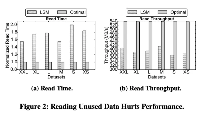
The evaluation results of both overall read time and read throughput are shown in Figure 2. Figure 2a illustrates that systems adopting the LSM-based strategy incur 1.53X ~ 2X longer read time than that of the optimal read case. This extra read time is caused by reading out 1.47X ~ 1.85X more data, where the data turns out to be unused. Moreover, reading un-needed data consumes additional bandwidth provided by SSDs and thus decreases effective bandwidth utilization. Based on our evaluation results shown in Figure 2b, the throughput of reading features from systems running the LSM-based strategy drops by around 22% ~ 31% compared with the optimal read case.

This work is strongly motivated by the urgent need to improve the read performance for recommendation training systems with SSDs. We propose a joint management middleware between recommendation systems and SSDs, so as to exploit unique access patterns of the recommendation model training (i.e. feature-based training) to facilitate the management of SSDs. Our ultimate goal is to:

1. Improve the read performance by reducing the amount of unused data.
2. Utilizing the high parallelism offered by SSDs.

The major technical challenge falls on:

1. How to eliminate the access behavior gap by pro-actively merging data belonging to the same feature without seriously hurting SSD’s lifetime.
2. how to improve SSD’s bandwidth utilization by smartly pinning data in the write buffer .

3 REC-AWARE SSD DATA ARRANGER

3.1 Overview

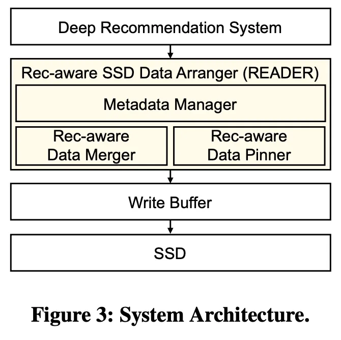
This section presents our rec-aware SSD data arranger (READER) to periodically rearrange KV-items stored inside SSDs with considering the recommendation model training behavior. As shown in Figure 3, READER is a middleware between the deep recommendation system and the SSD, and there is no modifications needed for both the recommendation training system and the FTL design inside the SSD.

• Section 3.2 presents two main data structures to keep track of the relation between each feature and its data arrangements in the SSD.
• Section 3.3 introduces the rec-aware data merger to merge scattered data belonging to the same feature.
• Section 3.4 then presents the rec-aware data pinner to improve bandwidth utilization by selecting frequently updated features and pinning data belonging to the features. Additionally, to avoid seriously hurting the lifetime of SSDs, updated KV-items will be buffered in the memory and appended to SSDs as a batch.

3.2 Metadata Manager

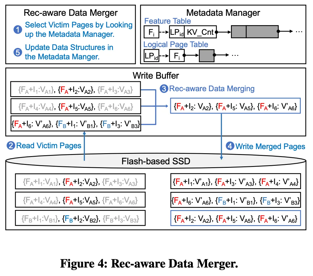
To bridge the access behavior gap between recommendation model training and the SSD, the metadata manager maintains two major data structures (as shown in Figure 4) to keep track of the relation between each feature and its data arrangements in the SSD, i.e., a feature table and a logical page table. Both of them are stored in storage devices and parts of these tables will be loaded and cached in memory on-demand for fast lookup.

The feature table is a hash table, where:

• key: a feature (i.e., $F_i$)
• value: a linked list

Each node in a linked list stores:

• an id of a logical page (i.e., $LP_{id}$) which accommodates KV-items belonging to the feature
• and a counter (i.e., KV_Cnt) to indicate the numbers of the KV-items in the page

FeatureTable = {
  F0 : LinkedList(
    Node(LP_id, KV_Cnt) -> Node(LP_id, KV_Cnt) -> Node(LP_id, KV_Cnt)
  ),
  F1 : LinkedList(
    Node(LP_id, KV_Cnt) -> Node(LP_id, KV_Cnt)
  ),
}

Please note that, the size of a logical page is aligned with the flash page size.

To obtain KV-items belonging to a feature, our middleware traverses the linked list to find all corresponding pages, reads out all these pages to memory, and then looks up KV-items inside these pages byte-by-byte .

This design can save a significant amount of space without maintaining an address for each KV-item especially when the size of an address is close to a KV-item. Even if each KV-item can attain an address, the corresponding page shall still be entirely read out because the minimum read granularity of an SSD is a flash page.

Thus, most of key-value databases designed for SSDs usually follow this design philosophy (e.g., LevelDB) to trade little read overhead for significantly minimizing the space requirements.

Additionally, controllers inside the SSD lack of the status information (i.e., valid or invalid) of each KV-item because both data updating and merging are controlled by our middleware outside SSDs. Thus, we also maintain a logical page table to keep track of the status information for each page.

The logical page table is a hash table, where:

• key: an id of a logical page (i.e., $LP_{id}$)
• value: is a linked list chaining all features (i.e., $F_i$) whose KV-items are stored in this page.

LogicalPageTable = {
  LP_id0 : LinkedList(
    Node(F0) -> Node(F2) -> Node(F5)
  ),
  LP_id1 : LinkedList(
    Node(F1) -> Node(F2)
  ),
}

When all KV-items in a page are marked as invalid:

1. Remove all nodes (aka. features) from the linked list.
2. READER notifies SSD’s FTL firmware to mark the corresponding physical page as an invalid page.

3.3 Rec-aware Data Merger

The proposed rec-aware data merger , as shown in Figure 4, is:

• Purpose: To merge scattered KV-items belonging to the same feature
• How to Achieve: exploiting the feature-oriented data structures maintained by the metadata manager. Our rec-aware data merger is activated when an updated KV-item is appended from the write buffer to an SSD.

As shown in Figure 4, there are two main stages of our data merger: (1) select victim features (❶), and (2) merge KV-items (❷ - ❺).

(Recall)

FeatureTable = {
  F0 : LinkedList({ LP_id, KV_Cnt } -> { LP_id, KV_Cnt } -> { LP_id, KV_Cnt }),
  F1 : LinkedList({ LP_id, KV_Cnt } -> { LP_id, KV_Cnt }),
}
LogicalPageTable = {
  LP_id0 : LinkedList({F0 -> F2 -> F5}),
  LP_id1 : LinkedList({F1 -> F2 -> F3 -> F4}),
}

To select a suitable victim feature, our data merger looks up the feature table and picks the updated features whose feature-fragmentation degree is higher than a threshold. The feature-fragmentation degree indicates the ratio between the overall size of flash pages occupied by all KV-items corresponding to the feature and the total size of these KV-items.

To avoid hurting SSD lifetime, instead of merging all KV-items belonging to victim features, our data merger will not merge KV-items located in the low-merging-benefit pages. A low-merging-benefit page indicates a page containing a lot of KV-items belonging to the victim feature .

Merging KV-items in the low-merging-benefit page has very limited improvement on read performance, but the merge traffics may degrade the lifetime of SSDs. Practically, our data merger judges whether a page is low-merging-benefit with regard to the feature by looking up the $KV_{Cnt}$ in the feature table.

After deciding the victim pages, our data merger reads out all victim pages from SSDs and merges KV-items belonging to victim features (❷ & ❸). Our data merger then writes the new merged pages to the SSDs, and updates both tables in the metadata manager (❹ & ❺).

3.4 Rec-aware Data Pinner

Gathered KV-items may be gradually mixed with other items belonging to different features until our data merger merges the feature again. We propose a rec-aware data pinner to avoid easily mixing KV-items belonging to different features during appending updated KV-items to SSDs. Our rec-aware data pinner:

• pins (or locks) updated KV-items belonging to a feature in the write buffer
• unpins items when the size of pinned items belonging to a feature reaches a threshold (e.g., 1/4 of flash page size).

With this design, items belonging to the same feature have higher probability to be stored in a same flash page so as to minimize reading unused data and improve the utilization of SSD’s bandwidth.

Specifically, our rec-aware data pinner pins updated KV-items belonging to features which have more KV-items in the write buffer. Practically, modern Linux kernel provides pin_user_pages() and unpin_user_pages() functions to pin and unpin user pages in the memory. Our data pinner maintains a rec-aware pin structure (as shown in Figure 5), which is a max-heap data structure, to keep track of new updated KV-items. Each node in the rec-aware pin structure contains two elements, the identification of a feature ($Feature_{id}$) and the number of corresponding KV-items (#Items) in the write buffer. The number of KV-items belonging to a feature is set as the key of the max heap structure.

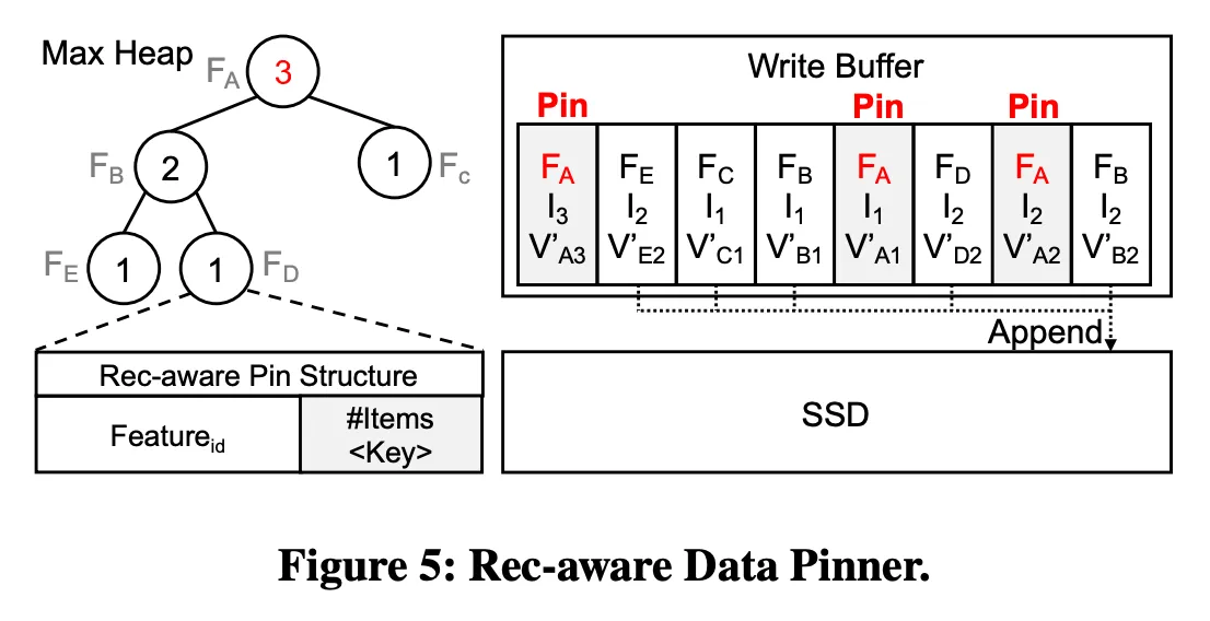
Figure 5 provides an example to show the interaction between our rec-aware data pinner and rec-aware pin structure. The rec-aware pin structure will be updated when an updated KV-item is added to the write buffer or appended to an SSD. Our rec-aware data pinner will select to pin KV-items belonging to the top-n features in the pin structure ($F_A$ in this example). After that, our data pinner calls the kernel function to pin KV-items (i.e., $\{F_A I_3 : V'_{A3}\}$, $\{F_A I_1 : V'_{A1}\}$ and $\{F_A I_2 : V'_{A2}\}$) related to selected features. Other non-pinned KV-items will than be appended to SSDs. Please note that, pinning too much items shrinks the available buffer size for new coming updated KV-items, and thus non-pinned KV-items belonging to different features will be mixed together easier. Based on our testing, to decide $n$ for top-$n$ features, we suggest to limit the overall pinning size to no more than 5% of the overall write buffer size .

graph LR
    A[新 KV item 進 buffer] --> B{屬於熱門 feature 嗎?}
    
    B -- "是" --> C[Pin 該 KV item]
    
    C --> D{湊滿閾值了嗎?}
    D -- 沒滿 --> C
    D -- 滿了 --> E[unpin 該 feature 所有 pages]
    
    B -- "否 (cold feature)" --> F[直接通過]
    
    E --> G[Merger 接手]
    F --> G
    
    G --> H[執行 Rec-aware Merge]
    H --> I[寫入 SSD]

4 PERFORMANCE EVALUATION

4.1 Evaluation Setup and Performance Metrics

This section evaluates the effectiveness of the proposed middleware for improving the feature reading performance of recommendation model training over SSDs, in terms of the overall read time and the SSD throughput .

We evaluate both metrics by comparing the proposed rec-aware SSD data arranger (denoted as “READER”) with two baseline approaches. That is, the LSM-based strategy (denoted as “LSM”), which is adopted in Baidu’s recommendation systems, and the optimal read strategy (denoted as “OPT”). In contrast to append updated data to SSDs, the optimal read strategy runs RMW operations to avoid mixing items belonging to different features in the same page.

Modern computer systems adopt write buffer to optimize the write operations. To provide further optimization for all approaches, all KV-items belonging to the same feature in the write buffer will be gathered and written to SSDs in a batch.

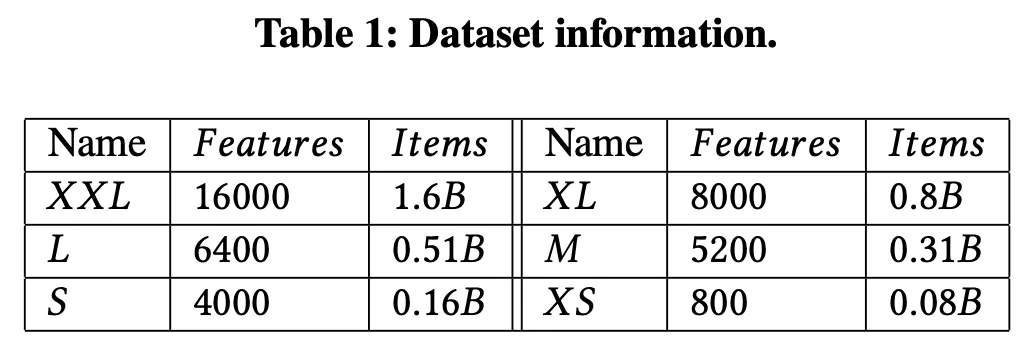
As shown in Table 1, we build six larger synthetic datasets by collecting multiple datasets from Kaggle (e.g., Goodreads-books, Top Games on Google Play Store, Hotel Recommendation, etc.). The extra extra large (XXL), extra large (XL), large (L), medium (M), small (S) and extra small (XS) datasets have around 1.6, 0.8, 0.51, 0.31, 0.16 and 0.08 billions of KV-items, respectively.

Experiment:

1. KV-items belonging to the same feature are written to the SSD in a batch.
2. Virtual write buffer: A suitable memory size (i.e., around 2.5% of the size of each dataset) is configured as a write buffer.
   • For example, the write buffer can buffer around 2 millions of the updated KV-items for the large dataset.
   • Please note that, we also provide results under smaller write buffer in Section 4.2.2.
3. The emulator uniformly selects and updates KV-items in a dataset.
   • Without loss of generality, the overall update counts are set to 800 millions to simulate that the systems have run for an enough long time.
4. Read out features from the SSD to train different models required by various web services
   • Totally read out around 60 thousands of features from the SSD.
   • Due to the fact that the same feature will be selected to train different models, the total features read from SSDs are more than the feature in each dataset.

Testbed of the Experiment

• Emulator runs on HPE server.
  • OS: Ubuntu 20.04.4
• CPU: Intel® Xeon® Gold 6252n
• DRAM: around 380 GB
• SSD: Intel DC S4500
  • Maximum Throughput: 540 MB/s
  • Use “FIO” (version 3.16) with 64 queue depths to sent requests to the SSD for measuring the overall read time and throughput.

4.2 Evaluation Results

4.2.1 Evaluation on Read Performance and Lifetime.

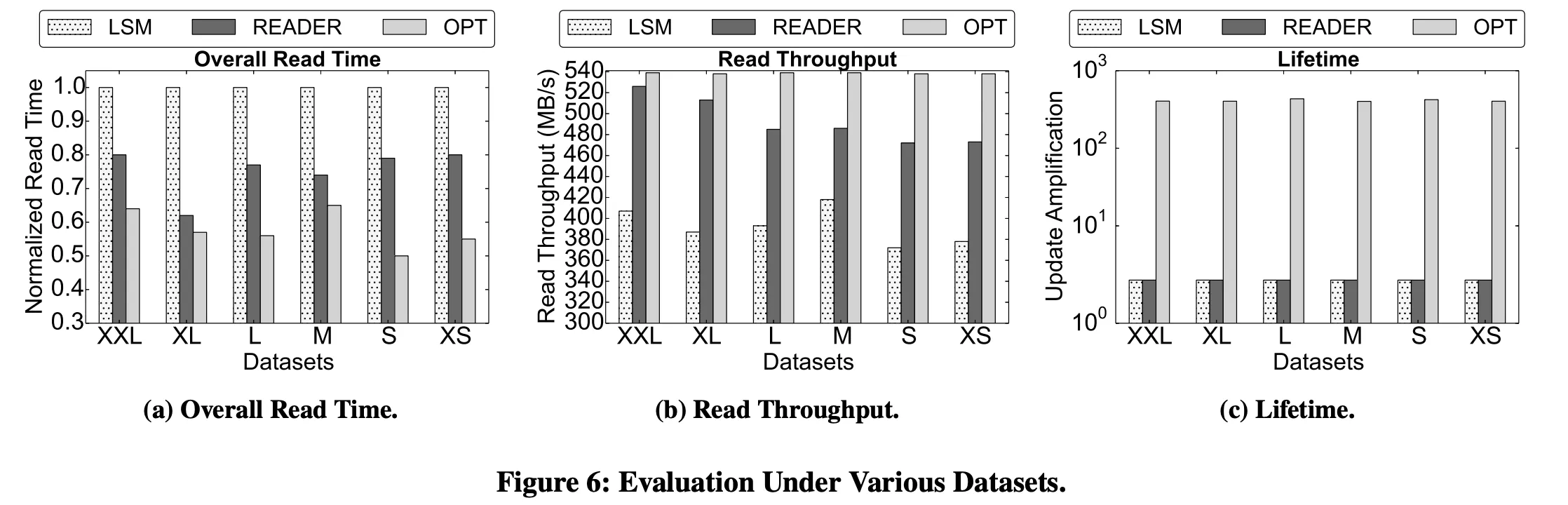
Figure 6 provides the results of the read performance and SSD lifetime under running READER against the LSM-based strategy and optimal read strategy.

Figure 6a shows the evaluation of the overall read time, where the x-axis indicates six datasets and the y-axis shows the overall SSD read time caused by reading required features. The results show that READER can save 20%~38% of overall read time compared with the LSM-based strategy . The reason is that READER manages the arrangement of KV-items in SSDs by considering the recommendation model training behavior. That is, READER gathers KV-items belonging to the same feature in a flash page. With running READER, systems read out fewer unused data during recommendation model training compared with systems running the LSM-based strategy.

Figure 6b shows the throughput evaluation where the y-axis shows the throughput of reading the required features from the SSD. The result shows that systems with running READER can reach 1.16X ~ 1.33X higher read throughput than the LSM-based strategy . The results imply that running READER has better utilization of SSD throughput than that of the LSM-based strategy. Moreover, with running READER, the throughput results are within 12% of the optimal read strategy .

Although the optimal read strategy can provide the optimal read performance, it may seriously hurt the lifetime of SSDs. Figure 6c shows the lifetime evaluation, where the y-axis shows the update amplification.

• Definition of update amplification: Amount of extra data written to SSDs for updating per KV-item in average.

The results show that the optimal read strategy requires around 400 times of extra writes for updating an item, and both READER and the LSM-based strategy only need 1 extra writes for updating each item . The results imply that running READER can improve around 400 times of SSD lifetime compared with using the optimal read strategy.

4.2.2 Read Performance under Smaller Write Buffer.

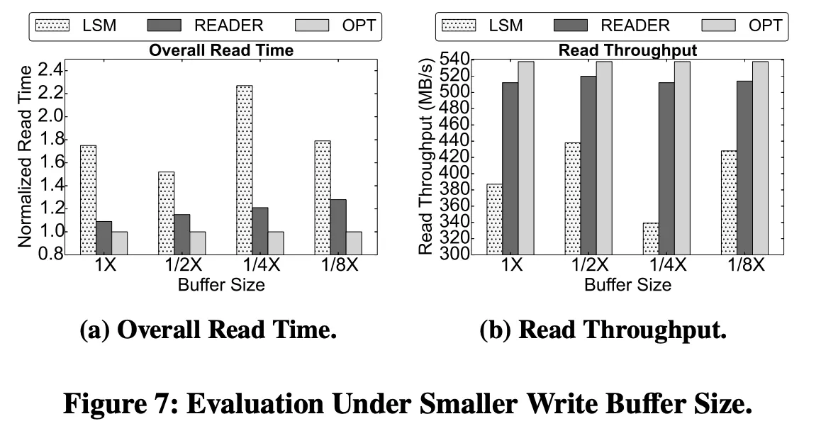
Figure 7 shows that READER is also effective and stable compared with the LSM-based strategy on systems with smaller write buffer. With considering the deployment costs, small and medium-sized enterprises or even personal customers may tolerate fewer performance degradation by shrinking the size of write buffer. Figure 7a shows the evaluation of overall read time on the XL dataset , where the x-axis shows the relative size of the write buffer compared with the size used by training the XL dataset and the y-axis shows the normalized overall read time. The results show that READER can save 24% ~ 47% of overall read time compared with the LSM-based strategy . Moreover, the design of the LSM-based strategy is not aware of the behavior of recommendation model training so that the overall read time seriously fluctuates . Figure 7b shows the throughput evaluation, where the y-axis shows the read throughput. The results show that READER can reach 1.19X ~ 1.51X higher read throughput than the LSM-based strategy .

5 CONCLUSION

Aiming for minimizing reading the amount of unused data from SSDs during recommendation model training, the paper presents a joint management middleware, namely rec-aware SSD data arranger (READER), to rearrange data in SSDs with considering the behavior of recommendation model training. READER comprises a rec-aware data merger to pro-actively merge data belonging to the same feature so as to avoid reading unused data from SSDs during training, and a rec-aware data pinner to smartly pin data in the write buffer so as to better utilize SSD’s bandwidth. The evaluation results show that running READER can save the overall read time by 20% ~ 38% compared with the LSM-based strategy, and our read throughput results are within 12% of the optimal case.

6 ACKNOWLEDGEMENT

We would like to thank Yunho Jin, Samuel Hsia, Udit Gupta, Mark Wilkening and Jeff (Jun) Zhang for their thoughtful comments and suggestions. This work was supported in part by the Ministry of Science and Technology, Taiwan, under Grant No. 110-2917-1-564-025, the Application Driving Architectures (ADA) Research Center, a JUMP Center cosponsored by SRC and DARPA.